Diffraction

Inspired by drudging through optics material for a recent exam, I wanted to get a more intuitive feeling for diffraction phenomena, specifically diffraction of spherical waves through a plane aperture.

Setup

The most general still-understandable way of calculating diffraction of such a configuration is the Kirchhoff diffraction formula. We assume at least one point source in a distance $z_s$ from the screen at $z = 0$, which emits a wave

\[\psi(\vec r) = \exp(i \vec k \cdot \vec R) \]

without any relevant time part, as we only care about a static setup.

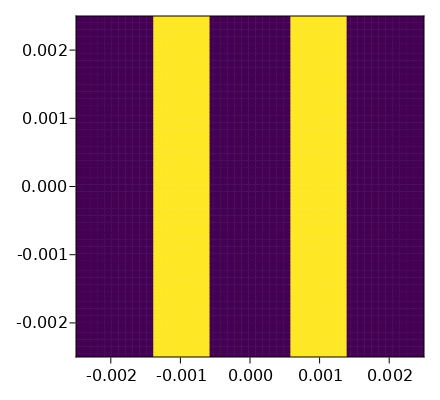
This wave arrives at the aperture ($z = 0$), and due to the Huygens principle, every “open” part in the aperture will emit secondary spherical waves. At some distance $z_d$ from the aperture, those waves will hit a screen and produce our diffraction image, which we are interested in calculating. Our illustrations below assume that the aperture is a double slit. That is, $\sigma$ is the area colored in yellow; all units are in meters:

Kirchhoff, Fresnel, Fraunhofer, Huygens, oh my…

The most accurate, but still understandable, diffraction integral is the Kirchhoff(-Fresnel) diffraction integral. It posits that the secondary wave $\psi’$ at a position $\vec r = (x,y, z_d)$ on the screen behind the aperture $\sigma$ is given by

$$\psi’(x, y, z_d) = -\frac{i}{\lambda} \int \int_\sigma \frac{\exp(i \vec k \cdot \vec R(\tilde x,\tilde y))}{R(\tilde x,\tilde y)} \frac{\exp(i \vec k \cdot \vec r(\tilde x,\tilde y))}{r(\tilde x,\tilde y)} \frac{\cos \alpha + \cos \beta}{2} \mathrm{d}\tilde x \mathrm{d}\tilde y $$

Wow! that’s a lot. But – it’s not that difficult to grasp. What we are doing is sum over infinitesimally small secondary waves across our aperture $\sigma$. Each of these waves consists of the primary part (the first term) emitted from the source over a distance $\vec R(\tilde x,\tilde y)$ to position $(\tilde x,\tilde y)$ within the aperture, and a secondary part from the same point $(\tilde x,\tilde y)$ in the aperture to a point $(x,y, z_d)$ on the screen ($\vec r(\tilde x,\tilde y)$). Then there is a (usually utterly insignificant) double-cos term accounting for the slant of a non-orthogonal wave incident (the wave then doesn’t contribute fully to the $z$-direction amplitude anymore). For our configurations, the angles $\alpha$ and $\beta$ between incident on aperture respectively screen were super small, meaning the term was mostly $=1$.

In front, there is a term $i/\lambda$, which is partly a phase factor ($i$ means a phase shift of 90 degrees of secondary waves with respect to primary waves), and accounting for the magnitude of secondary waves, which is proportional to $1/\lambda$.

This really is enough to do most calculations, with point sources at different positions, and the screen close or far. However, assuming mostly-plane primary waves and a long distance between aperture and screen, we can also use the Fraunhofer integral, which gives nicer results. “Nicer” because they are closer to what we would see with e.g. a Laser source. The Fraunhofer integral is then:

$$\psi’(x, y, z_d) = \int \int_\sigma \frac{\exp(i \vec k \cdot \vec R)}{R} \frac{\exp(i \frac{\vec k}{\lambda z} (x \tilde x + y \tilde y))}{r} \mathrm{d}\tilde x \mathrm{d}\tilde y $$

where $\vec R$ again is the connection between primary source and point $(\tilde x, \tilde y)$ in the aperture. This is the result of approximating the distances in first order. Another difference to the previous integral is that $r$ and $R$ are considered constant, although here they still show up explicitly.

Interestingly, if we further simplify the diffraction integrals, we arrive at something like

$$\psi’(x,y,z_d) = \int \int_\sigma \mathrm{d}\tilde x \mathrm{d} \tilde y A(\tilde x, \tilde y) \exp(-i \vec k \cdot |(x,y, z_d) - (\tilde x, \tilde y, 0)|)$$

as the diffraction pattern on the screen. You will notice that this is essentially a 2-dimensional Fourier transform, which “officially” is defined like this:

$$\hat f(\vec k) = \int \mathrm{d}^3 \vec x f(\vec x) \exp(-i \vec k \cdot \vec x)$$

But which function is being transformed? – it is the aperture function, meaning that what we see on the screen is the fourier transform of two rectangles. This result has always been amazing to me. In this figure you can see a purely mathematical 1D fourier transform of a double slit function (sketched in red). Notice the similarity to the plots shown below!

In any case – let’s get to the results!

Some pictures

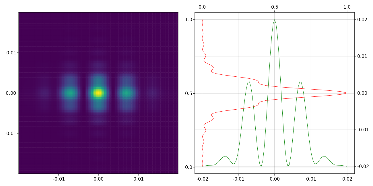
The double slit is a well-known experiment, so it’s suitable for evaluating whether our calculations were correct. It looks like it! On the right, we can see the cross section of intensities at $x = 0$ and $y = 0$ on the screen, respectively. As described above, we calculated a single point source in a great distance (compared to aperture dimensions) to the aperture, illuminating a screen that in turn was placed at a great distance from the aperture.

Kirchhoff diffraction

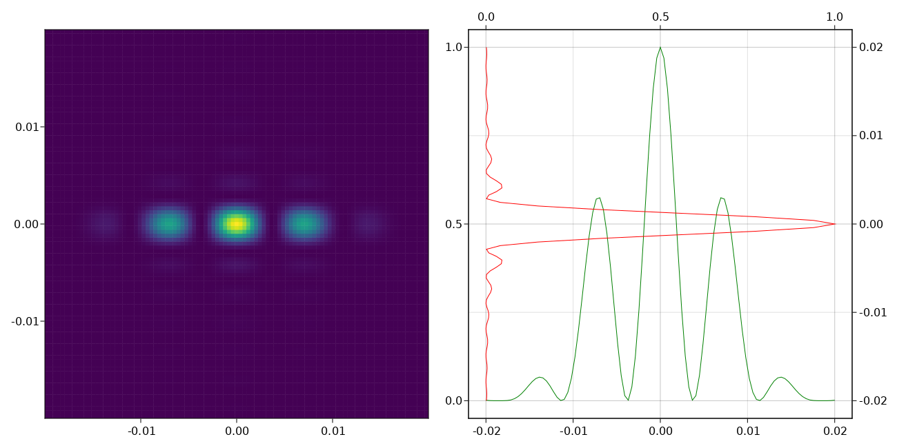
Fraunhofer diffraction This looks a bit more like the typical result with a laser, as we don’t get as much vertical diffraction.

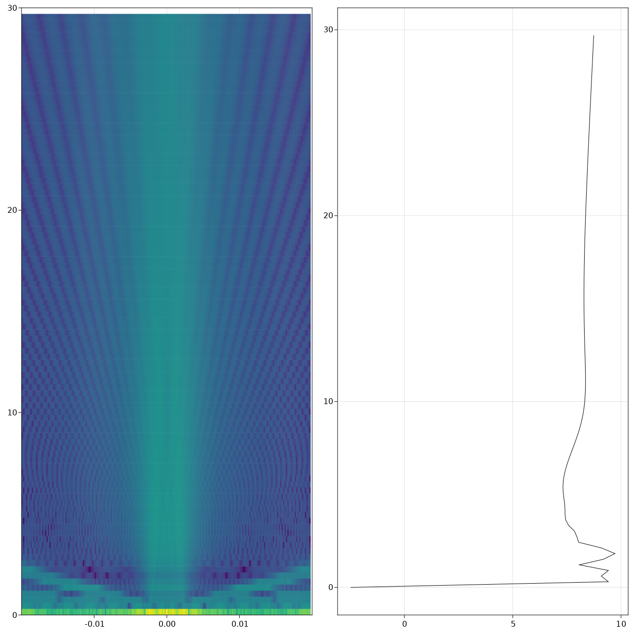
3D picture: how the waves propagate in the $x=0$ plane from aperture (bottom) to screen (up) on the right, log-intensity at $x = y = 0$

Calculation

The very core part is quite short. Calculated in parallel on four CPU cores, this algorithm takes only about 30 ns per iteration. That’s good because calculating the images above took 31049568 iterations per image. This algorithm only considers “lit” parts of the aperture, meaning that a sparse aperture will be much faster to calculate. In the worst case, the complexity is $O(n^2 m^2)$ where $n^2$ and $m^2$ is the number of pixels for aperture and screen, respectively. We return intensities on the screen together with a range of the sampled positions. That is what is then plotted in the images you see above.

Otherwise, there is not too much to say about this – it’s a very simple numeric 2D integration. We use an outer loop to integrate across the aperture $\sigma$, and an inner loop to integrate across the selected screen area, mapping each quasi-infinitesimal secondary wave to all positions on the screen. Some optimizations regard the calculations of cosines, which we approximate using the first order Taylor series ($\cos x \approx 1 - {x^2}/{2}$, good enough for our angles), and materializing our coordinates instead of keeping them as range (which greatly reduces the number of allocations to be done).

 1
 2
 3
 4
 5
 6
 7
 8
 9
10
11
12
13
14
15
16
17
18
19
20
21
22
23
24
25
26
27
28
29
30
31
32
33

function calculate_integral(setup::Setup; scan_param::ScanParam=default_scan_param)
    # Outer integral: dx dy -- sum across area elements
	@time begin for (apx, apy) = all_aperture_coords
		weight = setup.aperture(apx, apy; setup.aperture_kwargs...)
		if weight == 0
			continue
		end
		count += length(all_screen_coords)

        # prepare terms only dependent on aperture-(x,y)
		cdist = sqrt(apx^2+apy^2)
		dists = ((atan(sum(((s.x, s.y) .- (apx, apy)).^2)/abs(s.z)), 
					sqrt(sum(((apx,apy,0) .- (s.x, s.y, s.z)).^2)))
				for s = setup.source)
		sourceterms = [(fastcos(alpha), exp(-im * k * R)/R) for (alpha, R) = dists]
		
        # for this secondary wave, calculate contributions to every pixel on the
        # screen.
	    Threads.@threads for (i, scx, j, scy) = all_screen_coords
			pointdist = sqrt((apx-scx)^2 + (apy-scy)^2)
			r = sqrt(pointdist^2 + setup.screen_pos^2)
			beta = fastatan(pointdist / abs(setup.screen_pos))
			fcb = fastcos(beta)
			term = exp(-im*k*r)/r * sum(
					((fcb+fca)/2 * t
						for (fca, t) = sourceterms))
			
			screen[i, j] += weight * term * delta^2/(im*setup.lambda)
		end
	end
	end
	abs.(screen).^2, LinRange(-scan_param.screen_size/2, scan_param.screen_size/2, screendim)
end

The Fraunhofer integral is a bit easier. In any case, you can download the entire code as Pluto notebook from GitHub or as PDF. There are other pre-implemented aperture shapes for you to play with, such as circular apertures, square apertures, single slit, diffraction gratings, etc.